Image Classification and Performance measures

10 February 2021

Image classification is supervised learning [the process under human supervision] in the field of  AI and ML world and used to identify the objects [images] among others. Like Facebook and Google photos are examples of the most widely used.

Most of us know that these products can identify things, numbers, images of you, your friends and many more things around you.. But the question arises how?

Use cases:

• Facebook
• Google Photos
• surveillance and reconnaissance
• Theft alert
• Video content identification
• MRI studies and satellite imagery

Lets build a numerical character identifiable model using MNIST dataset.

MNIST

MNIST is a collection of small 70,000 images of digits written by employees of the US Census Bureau and highschool students. Images are labeled with the digit which it represents.

We have a set of target images and we will build a model which focuses on relying on patterns and inference to learn using labeled images as a training set.

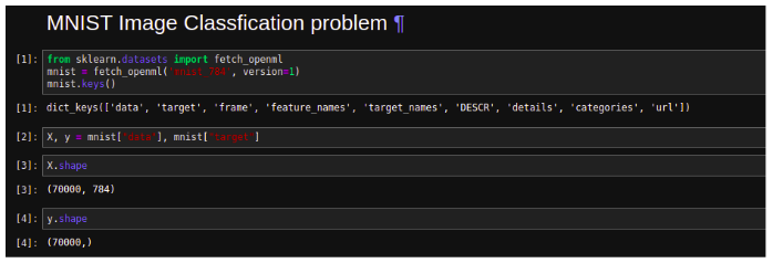
Import Dataset

Each images are of 28*28 pixels, so have 784 features and each feature has one pixel intensity from 0 to 255.

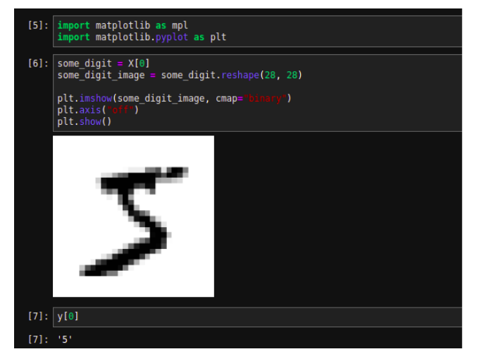
Let’s look at the very first image of this dataset.

Let’s cast the y as integer.

import numpy as np

y = y.astype(np.uint8)

Let’s create training and test sets. This dataset is already shuffled for us which guarantees that all cross-validation folds will be similar.

X_train, X_test, y_train, y_test = X[:60000], X[60000:], y[:60000], y[60000:]

Training a Binary Classifier

Let’s simplify the problem and identify the one digit only i.e a binary classifier with a Stochastic Gradient Descent (SGD) classifier, using Scikit-Learn’s SGDClassifier class .

y_train_5 = (y_train == 5) # True for all 5s, False for all other digits

y_test_5 = (y_test == 5)



from sklearn.linear_model import SGDClassifier

sgd_clf = SGDClassifier(random_state=42)

sgd_clf.fit(X_train, y_train_5)


sgd_clf.predict([some_digit])

Performance Measures

Measuring Accuracy Using Cross-Validation:

If you need more control on cross-validation process than what scikit-learn provides, then, you can implement cross-validation yourself.

from sklearn.model_selection import StratifiedKFold

from sklearn.base import clone

skfolds = StratifiedKFold(n_splits=3, random_state=42)

for train_index, test_index in skfolds.split(X_train, y_train_5):

clone_clf = clone(sgd_clf)

X_train_folds = X_train[train_index]

y_train_folds = y_train_5[train_index]

X_test_fold = X_train[test_index]

y_test_fold = y_train_5[test_index]

clone_clf.fit(X_train_folds, y_train_folds)

y_pred = clone_clf.predict(X_test_fold)

n_correct = sum(y_pred == y_test_fold)

print(n_correct / len(y_pred))

Output: # prints 0.9502, 0.96565, and 0.96495

The “StratifiedKFold” class performs the stratified sampling to produce the folds containing a representative ratio of each class.

Let’s make a classifier that just classifies every image in the “not-5” class

from sklearn.base import BaseEstimator




class Never5Classifier(BaseEstimator):

def fit(self, X, y=None):

return self

def predict(self, X):

return np.zeros((len(X), 1), dtype=bool)




Never_5_clf = Never5Classifier()

cross_val_score(never_5_clf, X_train, y_train_5, cv=3, scoring="accuracy")

Output: array([0.91125, 0.90855, 0.90915])

Confusion Matrix:

The general idea is to count the number of times where the instance of class ‘5’s’ are classified as ‘not 5’s’

from sklearn.model_selection import cross_val_predict

y_train_pred = cross_val_predict(sgd_clf, X_train, y_train_5, cv=3)




from sklearn.metrics import confusion_matrix

confusion_matrix(y_train_5, y_train_pred)

Output: array([[53057, 1522], [ 1325, 4096]])

The row of confusion matrix represents an actual class and the column represents the predicted class. Here the accuracy of +ve prediction is called precision of the classifier and the ratio of +ve instances that are correctly detected by the classifier is called recell or sensitivity or the true +ve rate.

Precision and Recall:

from sklearn.metrics import precision_score, recall_score

precision_score(y_train_5, y_train_pred)

Output: 0.7290850836596654

recall_score(y_train_5, y_train_pred)

Output: 0.7555801512636044

It is more convenient to combine precision and recall together into a single metric called F1 score.

from sklearn.metrics import f1_score

f1_score(y_train_5, y_train_pred)

Output: 0.7420962043663375

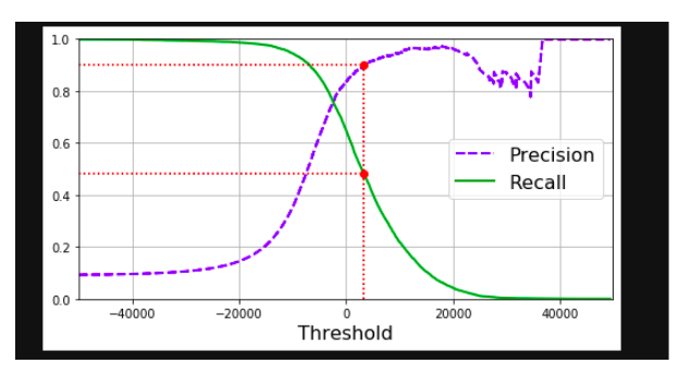
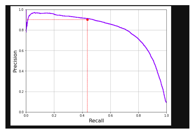
It always depends on the context that you want to precision or recall. Unfortunately, you can’t have it both, increasing the precision will reduce recall and vice versa and it is called the precision/recall trade-off.

Precision/recall trade-off:

The SGDClassifier makes its classification based on score from the decision function. If the score is greater than the threshold, it assigns that instance to the +ve class otherwise it assigns it to the -ve class.

We can’t set the threshold directly, instead we can use the decision scores that it uses to make the predictions. The default threshold is 0.

y_scores = sgd_clf.decision_function([some_digit])

y_scores

Output: array([2412.53175101])

threshold = 0

y_some_digit_pred = (y_scores > threshold)

Output: array([ True])

Increases the threshold to 8000

threshold = 8000

y_some_digit_pred = (y_scores > threshold)

y_some_digit_pred

Output: array([False])

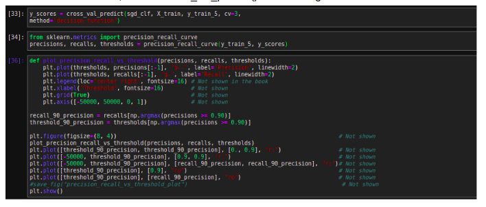
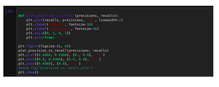
To decide the threshold, use the cross_val_predict() function to get the score of all instances.

Output:

The ROC Curve

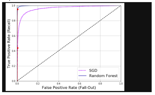
The receiver operating characteristic curve is another commonly used tool with the binary classifier. Instead of plotting the precision vs recall, the ROC curve plots the true +ve rate against the false +ve rate

Output:

The ROC AUC score

Another way to compare the classifier is to measure the area under the curve called AUC. The perfect classifier will have ROC AUC equal to 1

from sklearn.metrics import roc_auc_score

roc_auc_score(y_train_5, y_scores)

Output: 0.9604938554008616

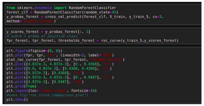
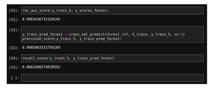
Now, use RandomForestClassifier and compare ROC curve and ROC AUC score to those of SGDClassifier.

Output:

Multiclass Classifier

Multiclass classifier (it is also called a multinomial classifier) can distinguish between more than two classes.

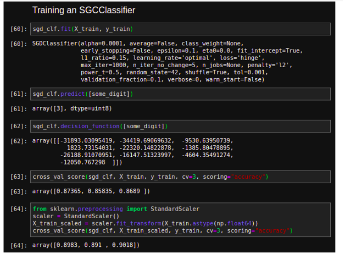
The Logistic Regression or Support Vector Machine Classifiers are strictly Binary Classifiers. However SGC classifier, Random Forest and naive Bayes classifiers are capable of handling multiple classes natively.

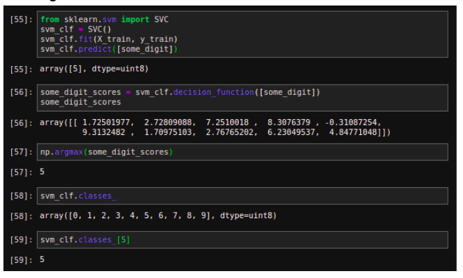
Training on SVC

Training an SGCClassifier with StandardScaler

Error Analysis

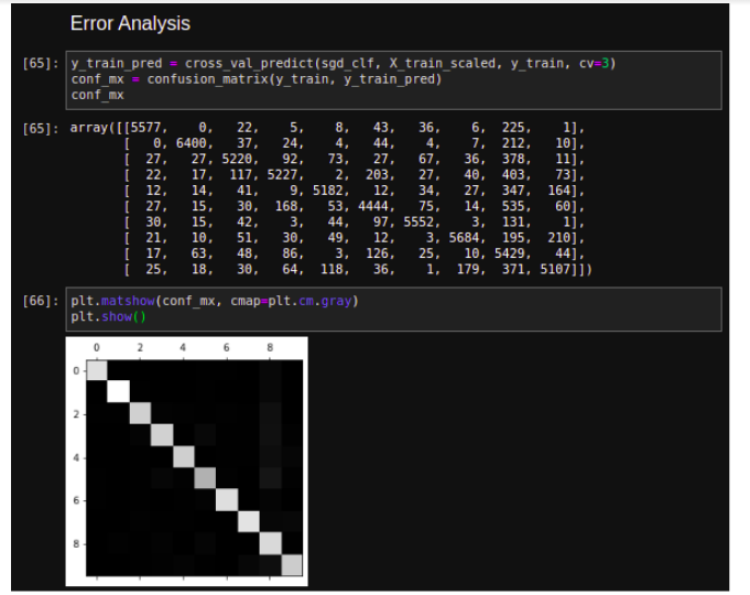
Let’s look at the confusion matrix, using the cross_val_predict() function, then call the confusion matrix() function

This confusion matrix looks great, since the most images are on the main diagonal, which shows that they were classified correctly. The fewer pixels are slightly darker than the others which shows that the classifier does not perform well on that pixel or image/digit.

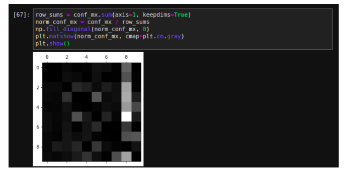
Let’s compare error rates instead of absolute numbers of errors

Now kind errors can be easily seen that the classifier can make. Remember, the rows represent the actual classes and columns represent predicted classes.

The column for class 8 is bright, which tells that the images get misclassified as 8s. However, the row for class 8 is not that bad, which shows the actual 8s get properly classified as 8s.

Multilabel Classifier

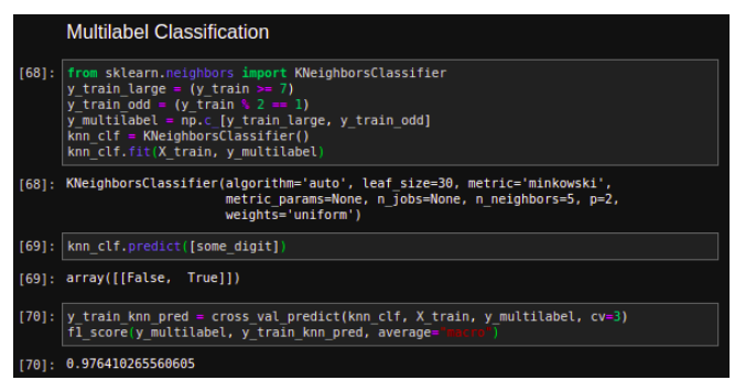
Until now each instance has always been assigned to just one class. But, in case you want to classify multiple classes for each instance like a face recognition classification, several people in the same picture. Such classification system that outputs multiple binary tags is called multilabel classification system.

Multi Output Classifier

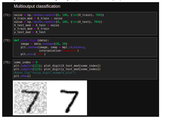
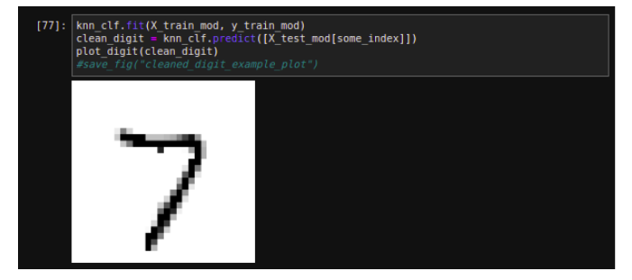
It is simply a generalization of multilabel classification where each label can be multiclass. It is also called multi-output-multiclass classification. Let’s build a system that removes noise from an image and output a clean digit image, represented as an array of pixel intensities.

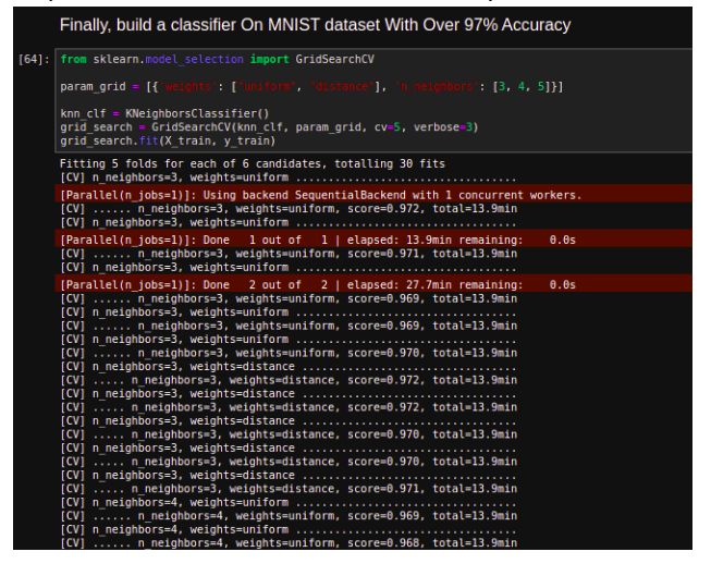
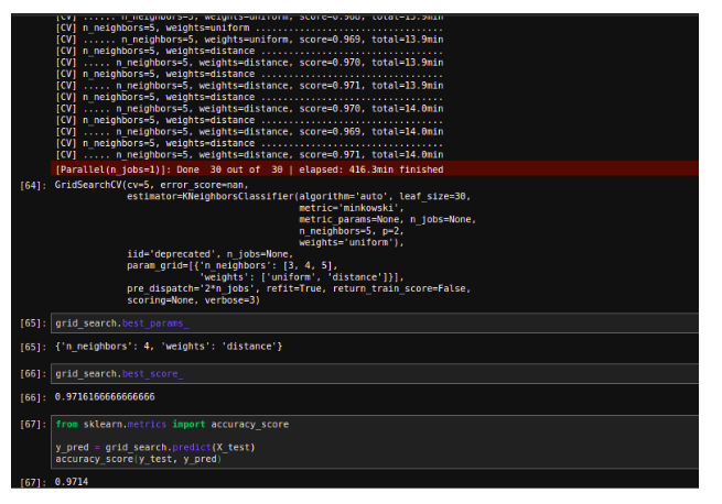
Finally, build a classifier On MNIST dataset With Over 97% Accuracy